Projected Gradient Descent with Skipping

During my time at IIT Madras, I had the incredible opportunity to attend a guest lecture by Prof. Sridhar Mahadevan, a distinguished researcher from University of Massachusetts Amherst. The lecture focused on acceleration in optimization methods, and one particular finding caught my attention that sparked this exploration.

Professor Mahadevan mentioned something curious about Runge-Kutta methods - that sometimes, when you look further ahead (higher order methods), you can actually get better convergence in fewer steps. This seemed almost counterintuitive at first glance, and I couldn't help but think there must be some trade-off involved.

This observation inspired me to investigate whether a similar phenomenon might exist in constrained convex optimization, specifically with projected gradient descent methods.

Constrained Convex Optimization

Consider the standard constrained optimization problem:

$\min_{x \in \chi} f(x)$

where $f$ is convex and $\chi$ is a convex constraint set.

Classical Projected Gradient Descent

The traditional projected gradient descent algorithm proceeds as:

$x_{k+1} = P_{\chi}(x_k - \eta \nabla f(x_k))$

where $P_{\chi}$ is the projection operator onto the constraint set $\chi$, and $\eta$ is the step size.

The K-Skip Projection Idea

What if we could skip some projection steps and still maintain convergence? I explored this idea by developing k-skip projected gradient descent variants.

2-Step Skip Projection

Instead of projecting at every step, we take two gradient steps and then project:

$y_{k+1} = x_k - \eta_1 \nabla f(x_k)$
$x_{k+1} = P_{\chi}(y_{k+1} - \eta_2 \nabla f(y_{k+1}))$

3-Step Skip Projection

Extending this further, we can skip even more projection steps:

$y_{k+1} = x_k - \eta_1 \nabla f(x_k)$
$z_{k+1} = y_{k+1} - \eta_2 \nabla f(y_{k+1})$
$x_{k+1} = P_{\chi}(z_{k+1} - \eta_3 \nabla f(z_{k+1}))$

The key insight is that we're taking multiple gradient steps in the unconstrained space before projecting back to the feasible region.

Experimental Results

I implemented these methods and tested them on constrained quadratic optimization problems. The results were quite interesting:

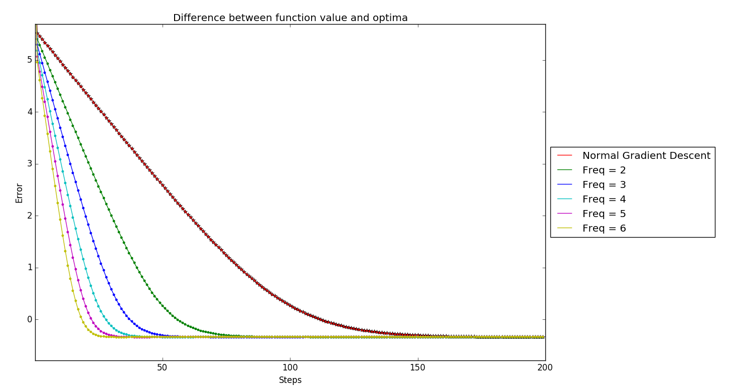
Key Observations

1. Improved One-Step Convergence: Methods with more skipping showed better convergence in the initial iterations
2. Different Convergence Points: Surprisingly, different k-skip algorithms converged to different points
3. Distance from Optimum: Higher skip orders tended to converge to points farther from the true optimal solution

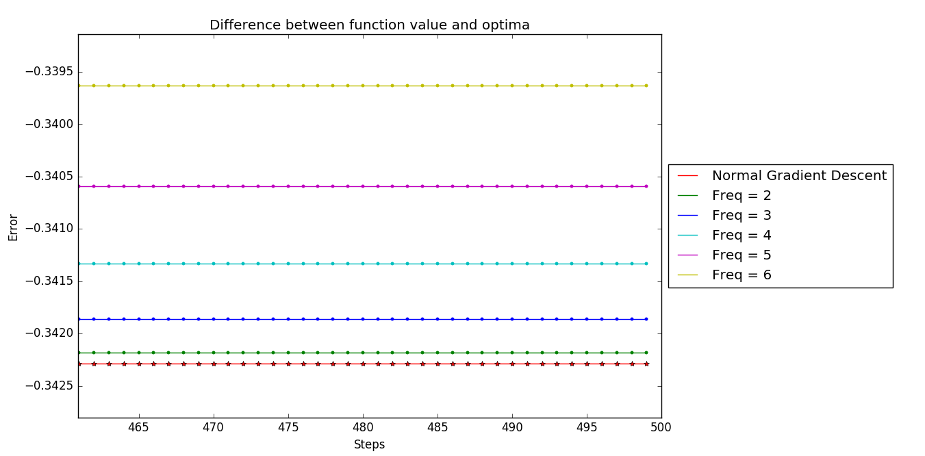
This zoomed view reveals the subtle but important differences in where each method ultimately converges.

Two Extreme Cases

The analysis revealed two interesting extreme cases:

1. Standard Projected Gradient Descent (k=0): Projects at every step
2. Infinite-Step Look-Ahead: Would be equivalent to solving the unconstrained problem and then projecting once

The trade-off becomes clear: while skipping projections can improve initial convergence speed, it may lead to convergence to suboptimal points.

A Potential Solution: Decaying Step Sizes

To address the convergence point issue, I experimented with decaying step sizes. The idea is to use larger step sizes initially (to benefit from the acceleration) and then decay them to ensure convergence to the correct optimal point.

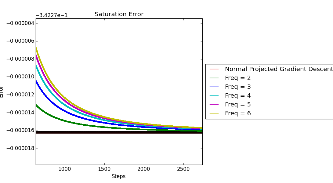
This approach showed promise in aligning the convergence points while maintaining some of the acceleration benefits.

Practical Implications

The main practical benefit of k-skip projected gradient descent could be in scenarios where:

1. Projection is Expensive: When computing $P_{\chi}(x)$ is computationally costly
2. Approximate Solutions Suffice: When you need quick convergence to a "good enough" solution
3. Warm-Start Available: When you have a good initial guess close to the feasible region

Future Directions

This preliminary exploration raises several interesting questions:

• Can we prove convergence guarantees for k-skip methods?
• What's the optimal choice of k for different problem classes?
• How do these methods perform with non-convex objectives?
• Can adaptive schemes automatically choose when to skip projections?

Conclusion

The investigation into k-skip projected gradient descent revealed an interesting trade-off between convergence speed and solution accuracy. While the initial results showed promise for faster convergence, the challenge of ensuring convergence to the correct optimal point remains.

This work demonstrates how ideas from one area of optimization (Runge-Kutta methods) can inspire novel approaches in another (constrained optimization). Sometimes the most interesting research comes from asking "what if we tried something slightly different?"

The complete analysis and code for these experiments can be found in my research notes, and I encourage others to explore this direction further.

---

This post is based on explorations conducted during my time at IIT Madras, inspired by Prof. Sridhar Mahadevan's insights on acceleration in optimization methods.