Projected gradient descent with skipping

One of the major benefits (among million others) of attending an elite university like IIT Madras is the various avenues it provides to get a glimspe into a world which you never knew of. Pursuing research and the thought of PhD was one such world which was brought within my grasp by IITM.

I was fortunate enough to attend one of the guest lecture by Prof. Sridhar Mahadevan , University of Massachusetts, during his visit to IIT Madras. He was going to discuss about his recent work (at that time) recent work with his student Ian Gemp . The plan of the talk (atleast to me) seemed to be : Start with variational inequalities and proceed to extragradient methods and state the results they worked out.

In the middle of the seminar, he said about a curious finding which pinged my interest. They had applied a logic based on Runge-Kutta methods to their problem and noticed that system kept converging faster and faster as the order of R-K method was increased. This was followed by a question by him,

So how much acceleration can we possibly obtain by including more and more terms?

This phenomenon irked me. According to my firm belief, there is always a trade-off. A system which just keeps providing improved one-step convergence without consequence? Something was definitely off.

My lifelong passion has been the theory behind optimization methods. Hence, I tried replicating similar situation (some would argue its exactly the same on some plane of thought) in constrained optimization using projected gradient descent.

Before diving deep into the exact question, a brief primer on the setup,

Constrained Convex Optimization

A simple constrained optimization problem of optimizing a convex function $f(x)$ over the set $x\in\chi$ can be stated as, $$\begin{equation} \min\ \ \ f(x)\ \ \ \ \text{over}\ \ \ \ x\in \chi \end{equation}$$

where assume that $f(x)$ is a doubly differentiable.

One of the go-to approach to solving the above problem is through projected gradient descent. The next iterate $x_{k+1}$ can we written as,

$$\begin{equation} x_{k+1} = P_{\chi}(x_{k} - \eta\nabla f(x_k)) \end{equation}$$

where the projection operator $P_{\chi}(x)$ is defined as, $$\begin{equation} P_{\chi}(x) = \arg\min_{y\in \chi}||x-y||^2 \end{equation}$$

Taking the que from Prof. Sridhar, consider the following iterations where we take projections on alternate steps as shown below. (I am calling it 2-step skip projection), $$\begin{equation} y_{k+1} = x_{k} - \eta_1\nabla f(x_{k})\end{equation}$$

$$\begin{equation} x_{k+1} = P_{\chi}(y_{k+1}-\eta_2\nabla f(y_{k+1}))\end{equation}$$

Similarly, we can consider a 3-step skip projection as well, $$\begin{equation} y_{k+1} = x_{k} - \eta_1\nabla f(x_{k})\end{equation}$$

$$\begin{equation} z_{k+1} = y_{k+1} - \eta_2\nabla f(y_{k+1})\end{equation}$$

$$\begin{equation} x_{k+1} = P_{\chi}(z_{k+1}-\eta_3\nabla f(z_{k+1}))\end{equation}$$

Further, we can keep increasing the number of skips to obtain any $k$-skip projected gradient descent.

Below is the error plot of these $k$-skip projected gradient descent for a simple example, where $error(k) = \log (f(Pr(x_k)) - f(x^*))$,

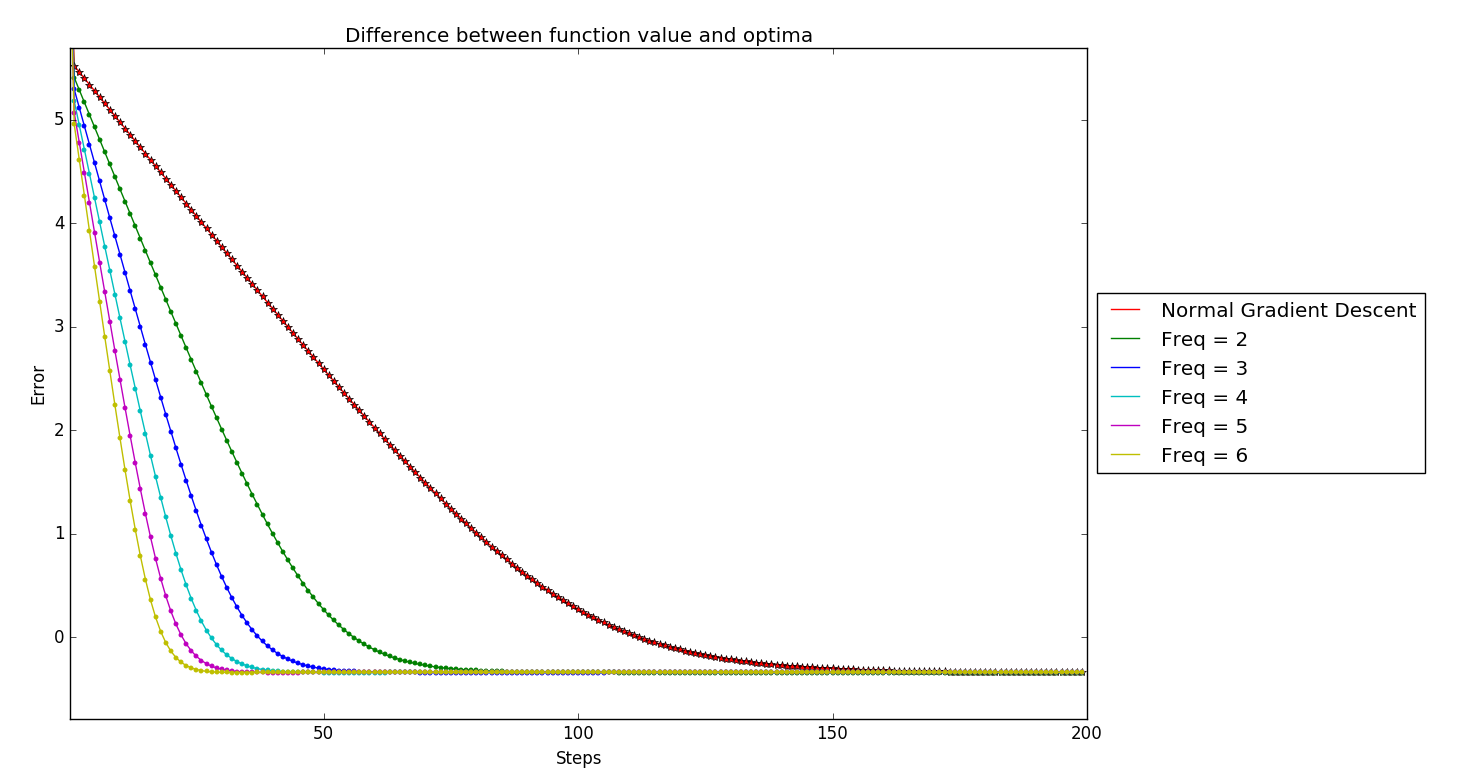
Initial thoughts

On first look, this experimental evidence confirms Prof.Sridhar’s claims!! More skipping just provides better one-step convergence.

But where is the trade-off? Lets look closely as to where the different $k$-skip algorithms are converging.

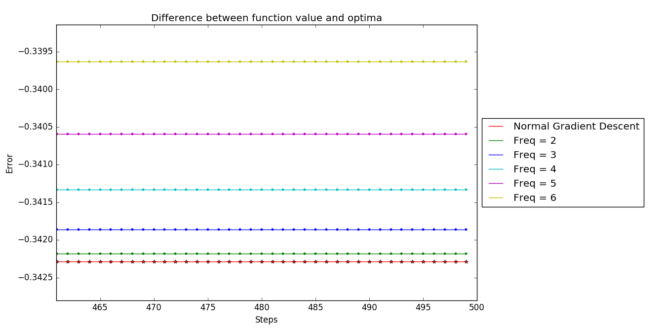
Note after enlarging the tail of the graphs, we can notice at all the distinct $k$-skip algorithms have distinct convergence point. And moreover, the more order of skip -> the farther away from the optimal solution (here optimal solution is the convergence point of standard projected gradient descent)

Why are we observing this?

The two extreme behaviour

We can consider the following high level view. Considering skipping with projected gradient descent, there are two extreme behaviour which can be thought of as follows:

1. Standard Projected gradient descent :

$$\begin{equation} x_{k+1} = P_{\chi}(x_{k} - \eta\nabla f(x_k)) \end{equation}$$

2. Infinite-step look-ahead gradient descent projection : The extreme case of $k$-skip algorithms will be when we are projecting only after we reach the optimal point $$\begin{equation} y = \arg\min f(x) \end{equation}$$

$$\begin{equation} x^* = P_{\chi}(y) \end{equation}$$ As noted in the sample simulations, the issue here is the difference in the fixed points in both these cases.

This provides a good intuition for the behaviour witnessed in tail-end of Figure 2.

Possibly Workaround

One easy and quick workaround to make sure that all the $k$-skip algorithms converge to the same point is to have decaying stepsizes i.e., we can make step-size (\eta) decay as $\frac{1}{t}$ which follows $\sum \eta_t = \infty$ and $\sum \eta_t^2 < \infty$.

Simulating the same setup with the new step-size routine, we obtain the following tail behaviour,

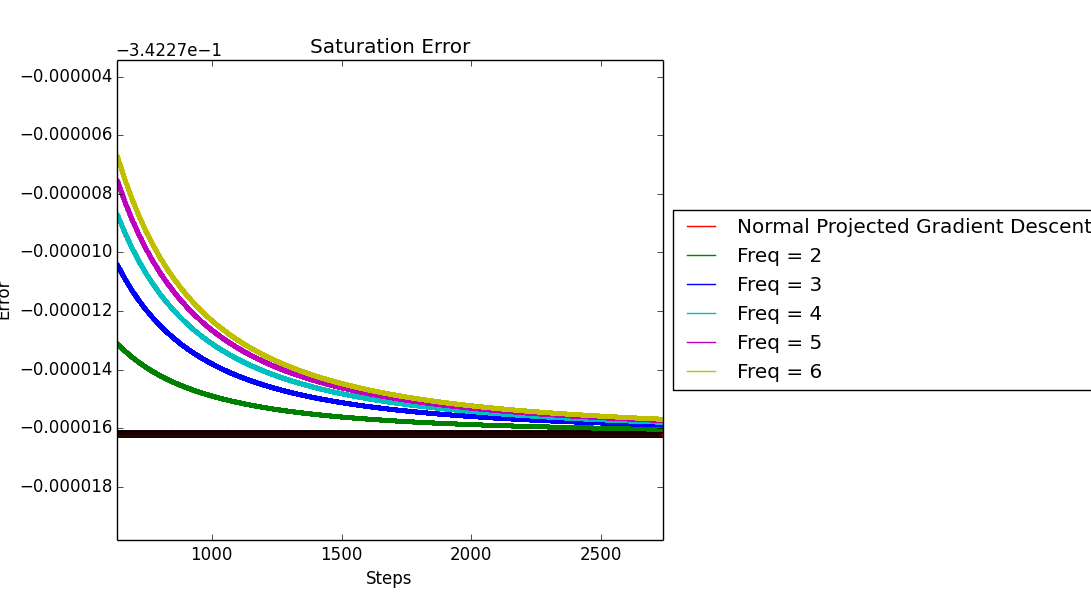
Benefits

In constrained optimization, one of the major computation issues concerning projected gradient descent is the projection step. Using the $k$-skip projected gradient descent reduces the total number of projections required by a multiplicative factor.

License

Copyright 2017 Parth Thaker .

Released under the MIT license.